CSCI 363 Computational Vision--Spring 2023
Assignments
Home | | Schedule | |
Assignments | | Lecture Notes
Assignment 1, Due Thursday, February 9
The aim of this assignment is to help you learn some of the basics of MATLAB
programming and begin thinking of 2D matrices as representations of images, with the
value at each location representing the light intensity at a corresponding position in
a 2D image.
Create an assign1 subdirectory inside the csci363 subdirectory
that you created for lab1,
and store all of your code files in the assign1 folder.
Further submission details are given at the end of this handout.
Problem 1: Create an image of blocks and circles
In MATLAB, it's easy to create an image with rectangular blocks of constant intensity.
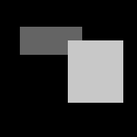
The following script creates an 8-bit gray-level image that has a background intensity of
0 and two overlapping blocks with intensities of 100 and 200:
% create an 8-bit image of size 200x200

image = uint8(zeros(200,200));

% add two rectangular blocks of constant intensity

image(40:80,30:120) = 100;

image(60:150,100:180) = 200;

imtool(image);     % display the image
 (1,1)
(200,1) |
|
 |
|
(1,200)
(200,200) |
We use uint8 (unsigned 8 bit integer) format to keep the size of the image files small.
The coordinates shown at the four corners of the above image are the pixel coordinates
(X,Y) printed
in the bottom left corner of the Image Tool display window. In pixel coordinates, the
location of the upper left corner of the darker gray block is (X,Y) = (30,40). In
the matrix indices, the order of the two dimensions is reversed, so the matrix location of
this upper left corner is image(40,30) (i.e. row 40, column 30, of the
image matrix). Carefully examine the relationship between the ranges of
coordinates in the above script and the position and size of the two blocks.
Part a: Making circles
Your first task is to write a MATLAB function named addCircle that adds a
circular patch of constant intensity to an input matrix. The function should have inputs and
outputs as shown in the following header:
function newImage = addCircle(image, xcenter, ycenter, radius, intensity)
Note that in Matlab, functions are written in the form:
	function output = functionName(parameterList)
	Code for body of function
	end
Whatever value is assigned to output by the end of the function execution
is the return value of the function. Thus the function call:
answer = functionName(parameterList)
will execute the function called functionName and the final value of output
will be assigned to answer.
Assume that the input image is a 2D matrix of uint8 values
that already exists. The circular
patch of intensity should be centered at pixel location (xcenter,ycenter)
and should have the specified input radius and intensity.
Your function can first alter the contents of the input image matrix to add
the new circle, and then copy the new contents of the image matrix into
newImage at the end of the function definition, using a single assignment statement:
newImage = image;
Alternatively, you can copy the original contents of the input image matrix into
newImage at the beginning of your function definition and then modify the contents
of newImage to add the circular patch.
When constructing the nested for loops to step
through the region of the matrix where the circle is added, think about how the range of values
for the control variables in the for statements can be specified in a way that
avoids unnecessary computations. For example, if you decide the outer loop will loop from the
minimum to the maximum Y values (what are these?), you will need to figure out the minimum
and maximum X values for each Y value to use as the range for the inner for loop.
Recall that for the outer edge of the circle, X^2 + Y^2 = R^2. So given Y and R
you can compute the max and min values of X. You can assume that this function will be called with
appropriate input values, so that the circular patch fits within the bounds of the matrix.
Store your new function in a file named addCircle.m in your assign1
folder. Be sure to place a semi-colon at the end of each statement that generates a value,
to avoid unnecessary printout during execution of the function. The following example
illustrates the application of this function:
image = uint8(zeros(200,200));

image = addCircle(image,80,50,30,100);

image = addCircle(image,150,100,20,200);
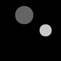
View your image using the command, imtool(image);
The first, larger circle is centered at pixel coordinates (80,50) and the
second, smaller circle is centered at pixel coordinates (150,100).
Part b: Creating color images
Color images can be stored in 3D matrices, where the third dimension stores the amount of
red, green and blue that combine to form a particular color. For example, load the
"peppers" image into MATLAB and view it with imtool:
peppers = imread('peppers.png');

imtool(peppers)
If you enter the whos command, you'll see that peppers is a
384x512x3 matrix of uint8 values.
The "Pixel info:" printed in the bottom left corner of the Image Tool window now displays
three intensity values corresponding to red, green and blue, e.g. [218 190 152].
You can use the Pixel Region Tool to examine the RGB values in image regions of different color.
A colorful RGB image of rectangular patches can be created by placing intensity values in
a 3D matrix, where the third dimension specifies color. The following example shows how
this idea extends to three dimensions:
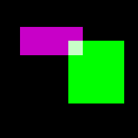
colorImage = uint8(zeros(200,200,3));    % create a 3D matrix

colorImage(40:80,30:120,1) = 200;     % add rectangle with a mix

colorImage(40:80,30:120,3) = 200;
% of red and blue

colorImage(60:150,100:180,2) = 255;      % add green rectangle

imtool(colorImage)
Matrix location colorImage(y,x,1) specifies
the amount of red that is displayed at pixel location (x,y), while
colorImage(y,x,2) specifies the amount of green and
colorImage(y,x,3) specifies the amount of blue displayed at pixel location
(x,y). In this example,
the upper left rectangle has red, green and blue values of 200, 0 and 200, respectively.
The mixture of red and blue creates the color magenta. The lower right triangle has red,
green and blue values of 0, 255 and 0, respectively, corresponding to pure green.
The overlapping region has a combination of all three colors, creating a whitish color.
Create a modified version of the addCircle function named
addColorCircle that adds a circular patch of constant color to an RGB image:
function newImage = addColorCircle(image, xcenter, ycenter, radius, r, g, b)
This function should assume that the input image is an existing 3D matrix of
uint8 values representing an RGB image. The circular patch of color should
be centered at pixel location (xcenter,ycenter) and should have the specified
radius. The input RGB values should be placed in the third dimension of the matrix.
Note that addColorCircle can be very similar to addCircle!
As a starting point, you can copy-and-paste your addCircle function into a new
M-File window in the MATLAB editor, save it in the file addColorCircle.m and then
modify the code as needed.
Problem 2: Blurring an image
One way to blur an image is to calculate the average intensity within a neighborhood of each
location. Write a function named blurImage that creates a blurred version of an
image using this technique. This function should have two inputs that represent the input
image and the size of the neighborhood, and a single output that is the new, blurred version
of the image. Assume that the input image is a 2D matrix of gray-level intensities ranging
from 0 to 255 (i.e. of type uint8). The output matrix should be the same size as
the input matrix, and can be created initially using the uint8 and
zeros functions. Suppose we let
nsize denote the input neighborhood size. Then the value stored in location
(x,y) of the output matrix should be the average of the intensities in the input
matrix calculated over a square region from (x-nsize,y-nsize) to
(x+nsize,y+nsize). This average can be converted to an integer using the
round function. You do not need to calculate average values for the region
of width nsize around the outer border of the image (these values can remain zero).
Note that the built-in sum function can be used to add the intensity values within
a square neighborhood around each location. You do not need to create an
additional pair of nested for loops to perform this step. Using sum on a
2D array will result in a 1D array with the sum of each column. Using sum on a 1D array
will result in a single number, which is the sum of the numbers in the array. Thus, the
call sum(sum(A)) will return the sum of all elements in the 2D array, A.
Test your function by
creating blurry versions of simple images that you create.
Problem 3: Finding edges
The images that you created in Problem 1a consist of patches of uniform intensity with sharp
intensity changes at their borders. The simplest way to find the edges in such images is to
scan each row of the image from left to right and look for a change of intensity between
adjacent pixels in the horizontal or vertical direction. Write a new function named
findEdges that has a single input that is a 2D gray-level image. This function
should return a 2D matrix of 8-bit values (i.e. with numbers of type uint8) of the same
size as the input image, which has the value 255 at the locations of edges in the input
image, and the value 0 elsewhere. To find the edges, the intensity at location
(x,y) can be compared to the intensities at locations (x-1,y) and
(x,y-1). If there is a difference of intensity in either direction, then 255
should be placed in the output matrix at location (x,y). You do not need to
detect edges along row 1 and column 1 of the input image. Test your function with simple
images that you create.
Submission details:
- Hand in a hardcopy of the files
addCircle.m, addColorCircle.m, blurImage.m,
	and findEdges.m
. To conserve paper, you can copy-and-paste the individual
code files into one extended M-File that you print out.
- Hand in your discussion log
- Upload to Canvas the following files:
addCircle.m, addColorCircle.m,
	blurImage.m, and findEdges.m
Home | | Schedule | |
Assignments | | Lecture Notes
Constance Royden--croyden@holycross.edu
Computer Science 363--Computational Vision
Last Modified: January 29, 2023
Page Expires: January 31, 2024