MATH 371 -- Numerical Analysis

November 14, 2001

Further Gaussian Quadrature Examples

First let's continue our work with

The Gaussian Quadrature approximation with

> f:=x->x^2/(1+x^2);

> x[5,1]:=-.9061798459:

> x[5,2]:=-.5384693101:

> x[5,3]:=0:

> x[5,4]:=-x[5,2]:

> x[5,5]:=-x[5,1]:

> c[5,1]:=.2369268850:

> c[5,2]:=.4786286705:

> c[5,3]:=.5688888889:

> c[5,4]:=c[5,2]:

> c[5,5]:=c[5,1]:

> GQ5approx:=add(c[5,j]*f(x[5,j]),j=1..5);

The exact value is

> Exact:=evalf(Int(f(x),x=-1..1));

> GQ5error:=abs(Exact-GQ5approx);

Let's compare this with the Simpson's Rule approximation using

the same number of function evaluations:

> with(student):

> Simpapprox:=evalf(simpson(f(x),x=-1..1,4));

> Simperror:=abs(Exact-Simpapprox);

As expected, the Gaussian Quadrature error is significantly smaller

(by an order of magnitude in this example).

Next, we show how to use Gaussian Quadrature over intervals other

than [-1,1]. For instance, let's see how to approximate

. First, we make the substitution

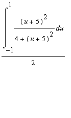
which takes the x- interval [2,3] to the u- interval [-1,1]. Under

this substitution, the integral to be computed becomes

> g:=u->(u+5)^2/(4+(u+5)^2)*(1/2);

> GQ5approx:=add(c[5,j]*g(x[5,j]),j=1..5);

> Exact:=evalf(Int(f(x),x=2..3));

> GQ5Error:=abs(Exact-GQ5approx);

This is much more typical of the behavior of the 5-point Gaussian Quadrature

error than the first example is!

> Simpapprox:=evalf(simpson(f(x),x=2..3,4));

> Simperror:=abs(Exact-Simpapprox);

>