MATH 241 -- Multivariable Calculus 

October 23, 2007 

The following plots show the graph of a function f(x,y), 

together with the graphs of its Taylor polynomials of degree 

1 and degree 2.    Here is the function  f 

(1)

 

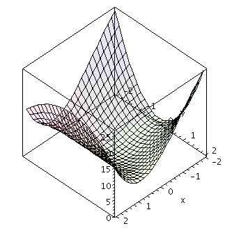
The graph of  f  alone: 

This computes the first degree Taylor polynomial at  (a,b) = (0,0): 

(2)

 

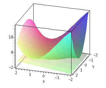
Here is the plot of  f  and the first degree Taylor polynomial.  The  

graph of  p1  is the tangent plane at  (a,b) = (0,0). 

This computes the second degree Taylor polynomial at  (0,0): 

(3)

 

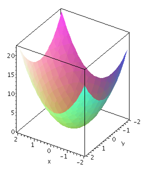
The graph of the second degree polynomial alone: 

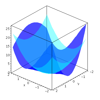
The graphs of  f  and its second degree Taylor polynomial together.