MATH 376 -- Probability and Statistics II 

A Comment on WMS, page 525. 

March 29, 2010 

I want to point out that there is a discussion in our text, Wackerly, Mendenhall,  

and Schaeffer, Mathematical Statistics with Applications, 7th edition, that is somewhat 

dated and that does not completely square with the current understanding in  

statistical science.  The statement in question is from the discussion of  

small sample tests for means on page 525 -- ``Such investigations [of 

the empirical distributions of the t-statistic] have shown that moderate 

departures from normality in the distribution of the population have 

little effect on the distribution of the test statistic''  -- a property 

called robustness.   This was certainly the consensus for a long time (say 

through the 1970's.)  However, more recent research has shown that 

this is not always the case  (or to be fair perhaps, that the precise meaning 

of ``moderate departures from normality'' needs to be more carefully stated!)   

How actually robust is the  t-test  in the case where the normality assumptions  

are violated? 

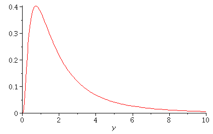
Let us study some small samples from a lognormal distribution.  (See the pdf 

plotted below.)  Note this is a skewed distribution with a relatively long right 

tail.   Many quantities observed in scientific experiments have distributions 

like this, so this is not just a theoretical example.   

(1)

 

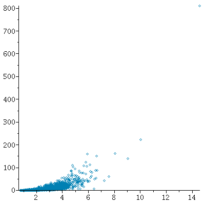
We generate 1000 random samples of size 8 from this distribution, and plot the means and 

variances of the samples in a scatter plot:





 

Recall that in the definition of  t-distributions, we said that when sampling from a
normal population,
 

             T =
had a  t-distribution with n - 1 degrees of freedom,  because it could be 

rearranged to put it into the standard form  , where  Z  is standard 

normal,  U  has a distribution with  n - 1  degrees of freedom, and  

Z  and  U  are independent.   This is the same as saying  Ybar  and  S  are 

independent.   Does that match what we are seeing with these 

samples?? 

Conclusion:  For these samples, it is not valid to assume that the sample mean and 

the sample variance (or standard deviation) are independent(!)   It is clearly true 

that the larger the sample mean is, the larger the sample variance is too. 

Does this make a difference??
 

(2)

 

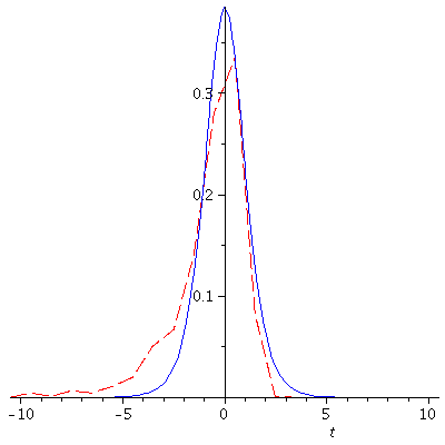
Now, let us compare the empirical distribution of the  t-statistics  from these samples 

with what we expect from the theoretical  t - density function:
 

 

	(3)

 

(4)

 

Note that the empirical distribution of the  t-statistics  is 

quite a bit different from the theoretical  t-PDF  for  

8 - 1 = 7 degrees of freedom.  The red empirical distribution  

has significantly more probability mass in the lower tail than 

the t-curve, and correspondingly less in the center and upper 

tail.  This means that confidence intervals or hypothesis 

tests using these samples will lead to incorrect conclusions 

more often than we expect.  (That is, for instance, the α and β 

for hypothesis tests will not achieve the desired values.) 

This kind of thing is more common than people thought until relatively 

recently.  Hence a whole new branch of the subject devoted to developing 

robust statistics (that is, statistics that are not overly affected by the  

failure of an assumption such as normality) has developed in the last 20 or 

30 years.  Our book, being an introduction to mathematical statistics, 

unfortunately does not discuss these methods.