MATH 136 -- Advanced Placement Calculus
An Euler's Method Example
November 18, 2009
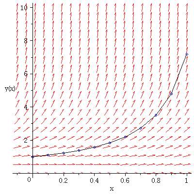
We study the approximate solution of ![]() =
= ![]() with initial
with initial
condition y(0) = 1. We do 10 steps of Euler's method with
![]() to approximate the solution at x between 0 and 1.
to approximate the solution at x between 0 and 1.
The Maple commands below execute the Euler's Method iteration
we discussed:
![]()
![]()
for the slope function ![]() starting from
starting from ![]()
| > | with(DEtools): |
| > | with(plots): |
| > | xlist[0]:=0; ylist[0]:=1; |
| (1) |
| > | for i to 10 do
xlist[i]:=xlist[i-1]+.1; ylist[i]:= eval(ylist[i-1]+(xlist[i-1]^2+ylist[i-1]^2)*(.1)); end do; |
| (2) |
| > | DirField:=dfieldplot(diff(y(x),x)= x^2 + y(x)^2,[y(x)],x=-.1..1,y=0..10): |
| > | Pts:=plot([seq([xlist[i],ylist[i]],i=0..10)],style=point,symbol=circle,color=blue): |
| > | Lines:=plot([seq([xlist[i],ylist[i]],i=0..10)],color=black): |
| > | display(DirField,Pts,Lines); |
 |
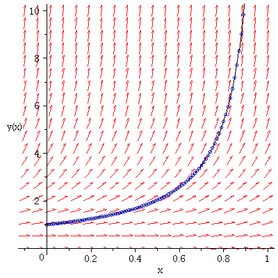
We would get a better approximation with smaller ![]() . For instance, with .01:
. For instance, with .01:
| > | xlist[0]:=0: ylist[0]:=1: |
| > | for i to 100 do
xlist[i]:=xlist[i-1]+.01; ylist[i]:= eval(ylist[i-1]+(xlist[i-1]^2+ylist[i-1]^2)*(.01)); end do: |
| > | Pts:=plot([seq([xlist[i],ylist[i]],i=0..100)],style=point,symbol=circle,color=blue): |
| > | Lines:=plot([seq([xlist[i],ylist[i]],i=0..100)],color=black): |
| > | display(DirField,Pts,Lines); |
 |
| > |